library(scienceverse)
#>
#> ************
#> Welcome to scienceverse For support and examples visit:
#> http://scienceverse.github.io/
#> - Get and set global package options with: scienceverse_options()
#> ************
# suppress most messages
scienceverse_options(verbose = FALSE)
Create the meta-study file
Once you’ve created a scienceverse study, you can set up a project from the meta-study file. Here’s a simple example testing group differences and simulating the data for the groups.
Simulate Data
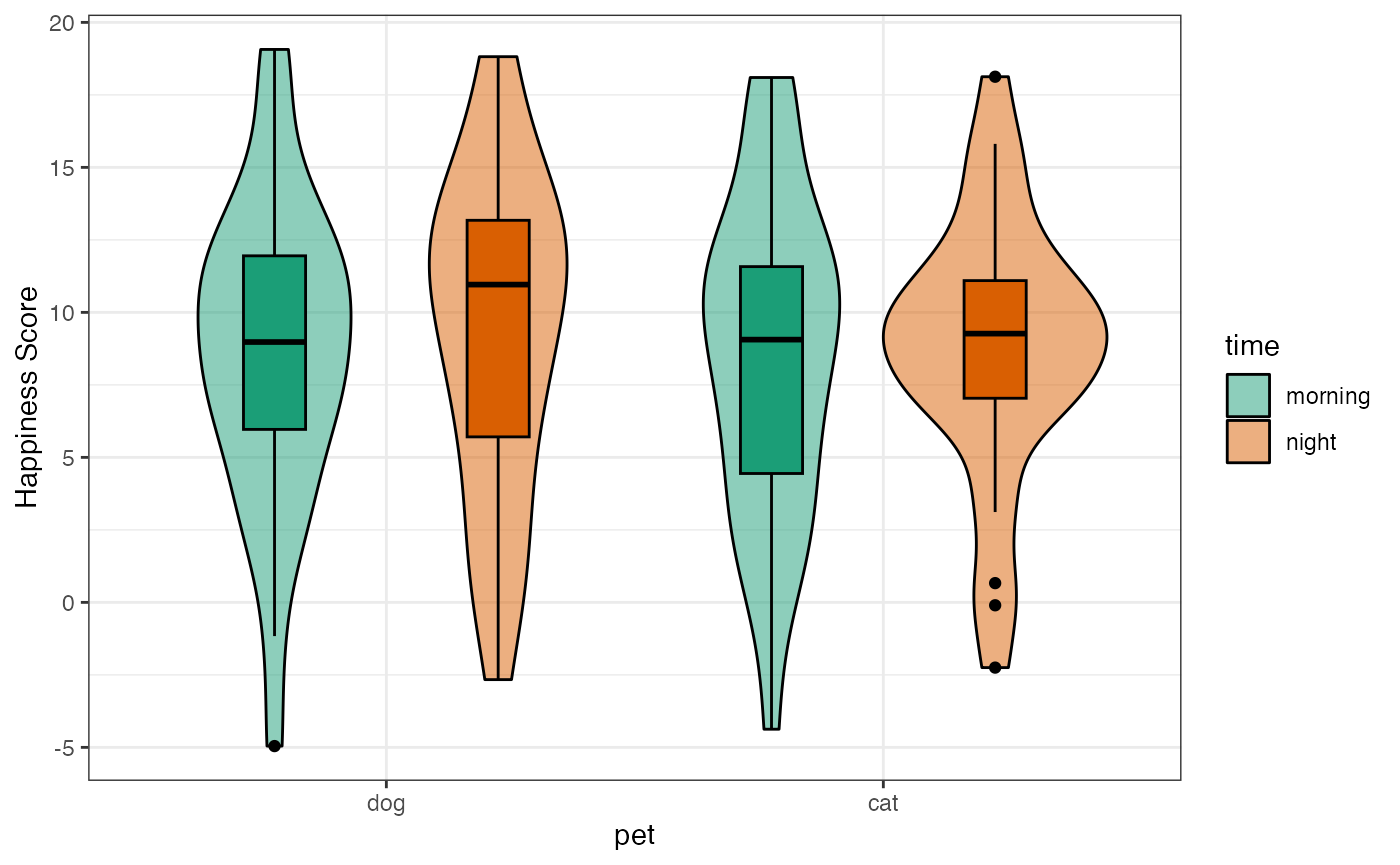
First, set up the basic study object and add a simulated dataset.
s <- study("Demo") %>%
add_sim_data("dat",
within = list(time = c("morning", "night")),
between = list(pet = c("dog", "cat")),
dv = c(y = "Happiness Score"),
mu = list(dog = c(10, 10),
cat = c(8)),
n = 30, r = 0.5, sd = 5, long = TRUE
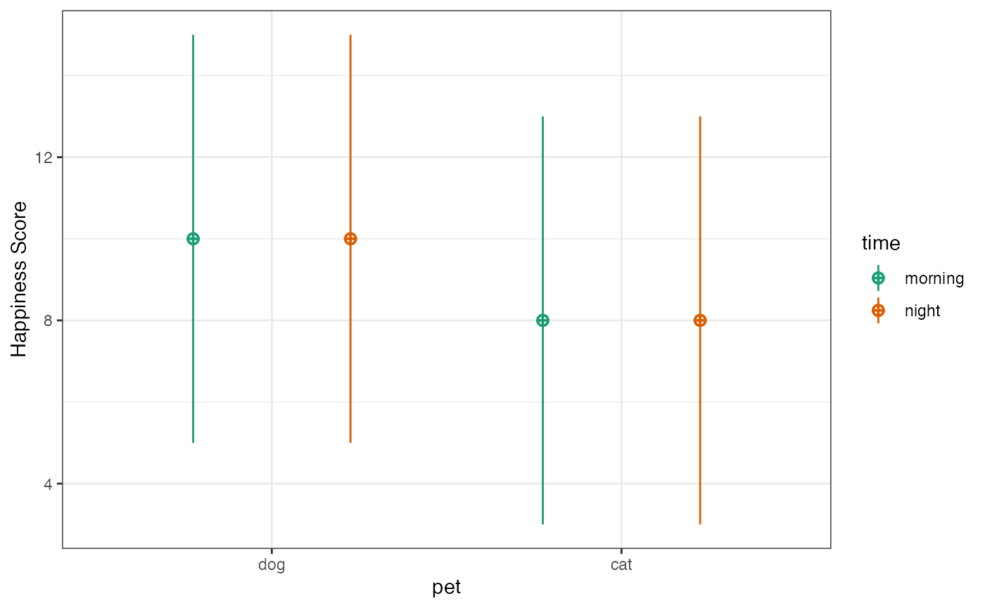
)Plot the actual data and the design to check it looks like you expect.
Set up hypotheses
Here, we’re adding two hypotheses, along with their associated analyses, evaluation criteria, and criteria for corroboration or falsification. These are very simple examples for demonstration, but you can include more complex analyses in curly brackets or as external .R files.
s <- s %>%
  add_hypothesis("group", "Dogs will be happier than cats") %>%
  add_analysis("A1", scienceverse::t_test(y~pet, dat)) %>%
  add_criterion("p", "p.value", "<", 0.05) %>%
  add_criterion("dir", "estimate[1]", ">", "estimate[2]") %>%
  add_eval("c", "p & dir") %>%
  add_eval("f", "p & !dir") %>%

  add_hypothesis("time", "Pets will be happier in the morning than at night") %>%
  add_analysis("A2", scienceverse::t_test(y~time, dat)) %>%
  add_criterion("p", "p.value", "<", 0.05) %>%
  add_criterion("dir", "estimate[1]", ">", "estimate[2]") %>%
  add_eval("c", "p & dir") %>%
  add_eval("f", "p & !dir") %>%
  study_analyse()
NB: I’m using the scienceverse function t_test() instead
of t.test because it gives you the Ns for each group in
between-group comparisons (useful for meta-analyses) and also labels the
estimates to avoid confusion.
Aftr you’ve run study_analyse(), printing the study
object will show a summary of the evaluation.
s
#> Demo
#> ----
#>
#> * Hypotheses: group, time
#> * Data: dat
#> * Analyses: A1, A2
#>
#> Hypothesis group: Dogs will be happier than cats
#>
#> Criterion p:
#> * p.value < 0.05 is FALSE
#> * p.value = 0.747
#>
#> Criterion dir:
#> * estimate[1] > estimate[2] is TRUE
#> * estimate[1] = 8.927
#> * estimate[2] = 8.620
#>
#> Conclusion: inconclusive
#> * Corroborate (p & dir): FALSE
#> * Falsify (p & !dir): FALSE
#>
#> Hypothesis time: Pets will be happier in the morning than at night
#>
#> Criterion p:
#> * p.value < 0.05 is FALSE
#> * p.value = 0.610
#>
#> Criterion dir:
#> * estimate[1] > estimate[2] is FALSE
#> * estimate[1] = 8.530
#> * estimate[2] = 9.016
#>
#> Conclusion: inconclusive
#> * Corroborate (p & dir): FALSE
#> * Falsify (p & !dir): FALSE
Save and reload
You can save the study in JSON (machine-readable) format and reload it later.
study_save(s, "study.json")
remove(s)
s <- study("study.json")
Get Results
You can get all the results with the get_result()
function. If you don’t specify the result name or the analysis ID, it
defaults to all of the results of the first analysis. It returns a list
that you can use, but will display an RMarkdown-formatted list if you
print it (and set the chunk options to results='asis').
get_result(s, analysis_id = "A1")- statistic: 0.3234
- parameter: 117.3873
- p.value: 0.747
- conf.int:
- -1.5737
- 2.1881
- estimate:
- 8.9267
- 8.6195
- null.value: 0
- stderr: 0.9498
- alternative: two.sided
- method: Welch Two Sample t-test
- data.name: y by pet
- n:
- 60
- 60
get_result(s, analysis_id = "A2")- statistic: -0.5117
- parameter: 117.5653
- p.value: 0.6098
- conf.int:
- -2.3653
- 1.3939
- estimate:
- 8.5302
- 9.0159
- null.value: 0
- stderr: 0.9491
- alternative: two.sided
- method: Welch Two Sample t-test
- data.name: y by time
- n:
- 60
- 60
Get a specific result from a specific analysis.
get_result(study = s,
           result = "p.value",
           analysis_id = "A2",
           digits = 3,
           return = "value")
#> [1] 0.61
Set return to “char” if you want to keep trailing zeros
(this returns the number as a character string).
get_result(study = s,
           result = "parameter",
           analysis_id = 1,
           digits = 5,
           return = "char")
#> [1] "117.38730"
Linked values
You can display the value as a link if you set return to
“html”. You can use the shorthand function get_html if you
only have one study object loaded. The digits default to the global
option, so you can set that as shown.
options(digits = 3)
get_html("p.value")
#> [1] "<a href='#analysis_1' title='Analysis 1 Result p.value'>0.747</a>"
You’ll probably want to use get_html() inline most of
the time like below. The links go to a section at the end of this
document that is created with make_script().
External analysis file
You can also display the value as a link to an external analysis file
created with make_script. For the shorthand function, set
the analysis link with scienceverse_options() as shown.
# create the analysis .Rmd and .html file,
# or you can do this outside this script
make_script(s, "analysis.Rmd")
rmarkdown::render("analysis.Rmd", quiet = TRUE)

scienceverse_options(analysis_link = "analysis.html")
get_html("p.value")
#> [1] "<a href='analysis.html#analysis_1' title='Analysis 1 Result p.value'>0.747</a>"
Here the inline links now go to an external file:
Inline Script
Add the script inline at the end with the function make_script. Set
header to FALSE to omit the YAML header. Set
header_lvl to change the default starting header level of
2.This function will save the data and codebooks in a folder called
“data”. Set the argument data_path to NULL to include the
actual data in the text of the script. For large datasets, you’ll want
to leave it as the default “data” folder (or set a custom folder
name).
make_script(s, header_lvl = 3, header = FALSE) %>% cat()